R For SEO Part 2: Packages, Google Analytics & Search Console With R
Hello and welcome to part two of my series on using the R programming language for SEO. Hopefully you enjoyed part one and are raring to go with today’s piece. Today, we’re going to be looking at R packages and as an example, we’re going to be using packages to directly pull in data from Google Analytics and Google Search Console. That’s right, no more downloading CSV exports and importing them.
If you find this useful, please consider giving it a share on your social networks and if you’d like to be kept up to date with my latest posts on this site, sign up for my free mailing list. No spam, no sales pitches, just updated content whenever it’s ready.
R Packages
I’ve mentioned this before in some of my other R blog posts, but packages are essentially plugins or extensions for the language. They’re a series of custom-built functions that are wrapped up and shared into one easily installable bundle and they’re often the quickest way to solve problems.
There are over 18,000 packages available on CRAN (the official R repository) and thousands more on GitHub and they’re a fantastic way to share or reuse your code. Although I won’t be covering how to build one in this series, it may be something I go back to later. It’s actually easy and I recommend creating a personal R package if you find you’ve got a lot of functions that you re-use. I have one myself and it’s saved me so much time.
As I say, I won’t be covering building your own R package in this piece, but there are several excellent resources below that you may want to check out as you get further on in your R journey:
- The Rstudio Package Dev Guide
- Hilary Parker’s Guide To Building A Personal R Package
- Hadley Wickham’s Advanced R Programming Guide To Packages
OK, now we know what an R package is, let’s install one.
The Tidyverse Package
With over 18,000 official R packages available, it can be a bit tricky to know where to start. As you get further into your R journey and start facing specific problems, you’ll become very familiar with Google and Stack Overflow. Nine times out of ten, you’ll find the answer there.
But for today, let’s install one package (or more accurately, a group of packages) that I almost never start an R project without: the incredible Hadley Wickham’s Tidyverse package.
I’ve long been an admirer of Mr Wickham’s work, particularly his dedication to making the R universe a better, tidier place and the Tidyverse package is essential. It incorporates the following other packages, which we’ll be becoming very familiar with the further we go through this series:
- ggpot2: The essential graphics and visualisation package for R
- dplyr: One of the most common and easiest to use data manipulation packages. We’ll be using functions from this one a lot
- tidyr: A fantastic series of functions for tidying up data sets. The more you do with R, the more familiar you’ll become with having to tidy up data, so this will become something you’ll use quite regularly
- readr: A package for reading rectangular data like CSVs, TSVs and other similar files
- purrr: A series of functions to help making working with functions and vectors easier
- tibble: Possibly the most annoying package ever created for people who don’t write clean code! Tibble is a new way of working with dataframes which, in Wickham’s own words “Does less and complains more” forcing you to write cleaner, more expressive code
- stringr: Another essential package for SEOs since we work with text data (strings) quite a bit and need quick, easy functions to deal with that
- forcats: This package offers a series of functions to make dealing with factors better or, frankly, tolerable
As you can see, there’s a lot in the Tidyverse that we’ll be using quite a bit as we go on through this series. So let’s get this installed for our first package installation.
Installing R Packages
Installing R packages is really simple once you know the name of the one you want to install.
As mentioned in the previous post on the basics of R, it’s always best practice to put your package installations into your .R file at the top of RStudio just so you can run the whole code back without trying to remember what packages you used. There are other options like Packrat, but since I work out of my Dropbox most of the time, this causes more problems than it solves for me, so I tend to just keep them at the top of my .R file.
In your text area, type the following:
install.packages("tidyverse")
Remember that R is case sensitive, so you’ve got to be accurate or else you’ll get an error.
Now add the following:
library(tidyverse)
Now paste these two commands into your RStudio console. You’ll see the following:

That’s it. Your Tidyverse package is installed and activated. The “install.packages” command downloads the package to your R environment and the “library” command activates it.
Unless you update your R installation, the installed package will stay installed and you’ll only need the “library” command to initialise it, but I recommend reinstalling regularly in case there have been updates.
Installing Multiple R Packages At Once
It’s nice to install our R packages as and when we need them, but if we know what packages we’ll be using at the start of our project, wouldn’t it be nice to cut down the lines we need to write? Here’s how you can install several R packages at once rather than numerous separate lines of code.
Firstly, we need to create a data frame containing the names of all the packages that we want to install. We’ll talk through the c( command in more detail shortly, but for now, just know it means “combine” and we’re going to create a list of the packages we want to install for this piece.
Rather than typing install.packages(“package”), library(package) like we did for the Tidyverse for every single package we want to use, if we know the packages we’re going to work with for our project, we can create a list like so:
instPacks <- c("tidyverse", "googleAnalyticsR", "searchConsoleR", "googleAuthR")
And then we can initalise them by calling the list with the Require command like so:
lapply(instPacks, require, character.only = TRUE)
If you know what packages you’re going to use at the start of your R project, or if you’re going to be running the same analysis for multiple clients, this is a great way to save time and make your code more efficient. It doesn’t work with every package, especially if you’re using them for the first time and there are authorisation requirements, or they’re coming from GitHub, but it’s always worth a try.
Now we’ve got our packages installed, let’s start getting some Google Analytics data directly into R using the googleAnalyticsR package.
Using Google Analytics In R
Now we’ve got our packages installed, we have to authenticate the googleAnalyticsR package with our Google Analytics account.
Here’s how to do that:
Authenticating GoogleAnalyticsR
First, type:
ga_auth()
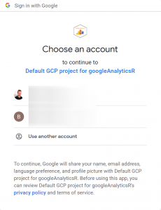
This will open a browser window with the following dialogue:

I’ve had some issues with this when the R version isn’t up to date, so make sure you’re always using the latest version of the language.
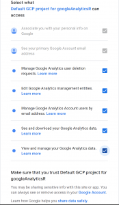
Make the following selections:

It will give you an authorisation code. Paste that into your R console
There you go, your R session is linked up with Google Analytics. Let’s get some data.
Querying Google Analytics Data In R With GoogleAnalyticsR
First, we need to create a dataset with our list of Google Analytics accounts and views. You can do that with the following command:
gaAccounts <- ga_account_list()
Now if you type
gaAccounts
in your console, you’ll get the full list of Google Analtyics accounts and views that are associated with the verified login you used. It’ll look something like this:

If you have multiple views and accounts in your Google Analytics account the way I do, you’re going to want to create an object with the view you want to work with. By looking at the table above (your own Google Analytics data will differ, obviously), we want to use the skills we learned in the previous post to explore our data and create an object in our R environment with it.
When you look through the output below, you’ll be able to identify the row number of the Google Analytics View you want to focus on. Once you know the row number, type the following:
viewID <- gaAccounts$viewId[ROW NUMBER]
Here, we’re creating a new R dataset with the specific row that we want to focus on from the viewID variable. When you look at the gaAccounts dataset, you should be able to identify the row number from the farthest left column. Put that number in the square brackets and your viewID data will be created, meaning you can use that instead of putting the specific number in with every API call.
Now we have that sorted, let’s make our first Google Analytics query in R.
Our First GoogleAnalyticsR Query
For a test, let’s just get sessions over the last seven days.
testData <- google_analytics(viewID, date_range = c("2022-02-01","2022-02-08"), metrics = "sessions")
At the time of writing this piece, that was the seven-day date range. Your mileage may well vary, but you can hopefully see how this works. Let’s break it down:
- testData <-: This is the name of our dataset. Since it’s just a test to make sure our connection is working properly, we’re just calling it “testData” for now
- google_analytics(: We’re telling R that we want to use the google_analytics function from the googleAnalyticsR package, we’re going to be downloading data from Google Analytics
- viewID: We’re invoking the viewID data that we created in the previous section, telling googleAnalyticsR what Google Analytics view we want to query
- date_range =c(: The date range we want to query. The c( command means “Combine”, something we’ll be using a lot more as we go. In this case, we’re going to combine our start and end dates
- metrics=: The metrics from Google Analytics that we want to get our data from. In the case of our first query, we just want to get “sessions”, but in the next section, we’ll be gathering more
If everything’s gone to plan, typing the following into your console:
testData
Will bring up the following:

Great, so we know it works. Now let’s get some more data and make it SEO-specific.
Multiple Metrics In GoogleAnalyticsR
First, we want to start building our query to include multiple metrics to look at our website’s performance.
Let’s get Sessions, Users, Pageviews and Bounce Rate.
GAData <- google_analytics(viewID, date_range =c("2022-02-01","2022-02-08"), metrics = c("sessions", "users", "pageviews","bouncerate"))
Again, there’s that c( command again. In this case, we’re telling Google Analytics that we want to combine all these metrics into a single dataframe.
If we run it using GAData, we’ll see the following:

Nice to see, but not particularly useful. Let’s start breaking it down a bit with dimensions and segments.
Adding Segments In GoogleAnalyticsR
Since this whole series is about using R for SEO, it makes sense that we’d start pulling our Google Analytics data using the organic search segment. Here’s how we can do that.
There are a couple of steps to this. First, since every Google Analytics account may well be different, we need to find the ID of our organic segment. On top of that, going forwards, you may want to get the IDs of other segments you have, so it makes sense to create a dataframe of them all. You can do that like so:
GASegments <- ga_segment_list()
Now our gaSegments dataset has all the IDs of the segments in our Google Analytics account. Look through that dataset using the gaSegments command in the console to find your ID, or search for it using the following command:
which(GASegments$name == "Organic Traffic")
From here, whichever route we go, we know the ID of our organic search segment. In my case, it’s 5. Now we need to define that segment for googleAnalyticsR. You can do that like so:
orgSegment <- segment_ga4("orgSegment", segment_id = "gaid::-5")
This has been a bit of a mission for the first run, but now we’ve got our organic search segment defined in R, we can work that into our original query like so:
GADataOrg <- google_analytics(viewID, date_range =c("2022-02-01","2022-02-08"), metrics = c("sessions", "users", "pageviews","bouncerate"), segment= orgSegment)
Take a look at it by typing GAData into the console.
And there we go. We’ve got the same dataframe as before, but using just organic search data. You’ll notice the “Segment” header added to the frame.
Now let’s break it down by the date dimension so we can see some performance trends.
Adding Dimensions To GoogleAnalyticsR
To break your Google Analytics data down by dimension in R, we just need to add the dimension parameter to our Google Analytics query, like so:
GADataOrgDates <- google_analytics(viewID, date_range =c("2022-02-01","2022-02-08"), metrics = c("sessions", "users", "pageviews","bouncerate"), dimensions = "date", segment= orgSegment)
Now you can see your performance over that date range using the organic segment, but we don’t want to figure out the date ranges manually every time, do we? Let’s see how to make the date ranges dynamic for every time we call it.
This will be important for later pieces in this series, and we’ll be covering other dimensions as well, so if you’re not familiar, it’s worth taking a look at the Google Analytics dimensions list.
Using Dynamic Date Ranges In GoogleAnalyticsR
This is actually quite easy, but wasn’t immediately obvious to me from the documentation when I first started using googleAnalyticsR, so hopefully this helps.
First, we need to edit our query using the c( parameter, but saying how many days we want to cover using the API shortcuts, like so:
GADataDynamicDates <- google_analytics(viewID, date_range =c("7DaysAgo","yesterday"), metrics = c("sessions", "users", "pageviews","bouncerate"),dimensions = "date", segment= orgSegment)
As you can see, there are options here. There’s a lot of flexibility available if you use the following API shortcuts.
And there we have it, a rolling date dimension in googleAnalyticsR, using the organic search segment. Again, this is something that we’re going to be using a lot more as we go through this series, so it’s worth getting familiar with it now. And be sure to save this dataset, because we’re going to be using this as a basis for the next few posts.
Now let’s take what we’ve learned about using R packages and Google APIs to the Google Search Console R package, searchConsoleR.
Using Google Search Console In R
The searchConsoleR package has a lot of great features and it’s pretty easy to use as well, so that’s what we’ll use to work with Google Search Console in R.
As with the googleAnalyticsR package, we need to authorise the R environment with our account. We can do that with the following command:
scr_auth()
As with googleAnalyticsR, it’ll give you an authorisation option in your console window and then open a new browser window. I don’t generally install the httpuv package as I change accounts so often with this, but your mileage may vary.
Allow access to your chosen Google account and you’ll see an authorisation code. Paste this in and you’ll see a message in your console saying you’re authorised.
OK, now we’re linked up, let’s get some data.
Getting Google Search Console Data With SearchConsoleR
The searchConsoleR package gives you a wide range of functions, including rewriting your data, deleting sites and much more, which are a bit beyond the scope of this series, since we’re just looking at how we can use R for SEO-specific data analysis, but there’s lots covered in the documentation.
As an example, let’s get our Google Search Console data for the last seven days. We can do that like so:
scData <- search_analytics("https://www.ben-johnston.co.uk", startDate = Sys.Date() -7, Sys.Date() -1, searchType = "web")
You’ll get a warning that Search Console data isn’t accurate for the last three days, but it’ll still give you something to work with. If you’ve been working in SEO for more than fifteen minutes, you’ll know that Search Console data is not what you’d describe as reliable at the best of times, so this isn’t a huge shock. That aside, let’s break the query down:
- scData <-: What we’re naming our dataset
- search_analytics(: We’re calling the search analytics part of the API, allowing us to get Google Search Console performance data
- “https://www.ben-johnston.co.uk”,: The name of the website we want to work with. You’ll need to put the full URL in there. I’ve used this site for this example
- startDate = Sys.Date() -7,: The Search Console API doesn’t have the same shortcuts as the Google Analytics API, so we need to be a little bit sneaky to get our rolling date ranges. Here, we’re using the Sys.Date() command to get the computer’s date and -7 to tell it to start seven days ago
- Sys.Date()-1,: As above, we’re telling the API call that the end of our date range is the computer’s date to yesterday
- searchType = “web”): We’re ending our API call by telling Search Console which type of search we want to look at. Obviously, Search Console breaks the different searches down by search type, so there are options here. I’m just using “web” for this example
If this runs correctly, you’ll get a dataframe like so:

Handy, right? Much quicker than downloading it manually. But not that helpful if we want to look at performance trends. Let’s look at how we can add dimensions to it.
Using Dimensions In searchConsoleR
As with the Google Analytics API, we can use dimensions to break our Google Search Console queries down.
As we all know, Google Search Console doesn’t have quite as much flexibility as Google Analytics, but hopefully by using dimensions, you’ll get some ideas of how you can use Google Search Console with R.
The dimensions available in the searchConsoleR package are:
- date
- country
- device
- page
- query
- searchAppearance
Now we have our list, let’s apply a date dimension to our data.
Using Date Dimensions In searchConsoleR
As with our googleAnalyticsR queries, if we want to add a dimension to our Google Search Console R query, we need to add the “dimension” parameter to our command. We can do that like so:
scDataByDate <- search_analytics("https://www.ben-johnston.co.uk", startDate = Sys.Date() -7, Sys.Date() -1, searchType = "web", dimensions = "date")
You’ll notice that nothing’s changed apart from adding the “dimensions = “date” parameter to our original call, which we discovered in the previous section. From running this, we’ll get the same dataframe as above, but broken down by date like so:

Wrapping Up
And there we go. We’ve learned how to install and initialise R packages and had a tour of the main Google Analytics and Google Search Console R packages. Remember to save your script from this piece, because we’re going to be using these datasets in the next few articles.
As always, if you have any questions, drop me a line on Twitter or through the contact form, and I’ll see you in a few days for the next piece, where we’ll talk about SEO data visualisation in R.
Our Code From Today
## Install Single Package

install.packages("tidyverse")

library(tidyverse)

install.packages("googleAnalyticsR")

library(googleAnalyticsR)

install.packages("searchConsoleR")

library(searchConsoleR)

install.packages("googleAuthR")

library(googleAuthR)

## Installing Multiple Packages

instPacks <- c("tidyverse", "googleAnalyticsR", "searchConsoleR", "googleAuthR")

lapply(instPacks, require, character.only = TRUE)

## Authorise Google Analytics

ga_auth()

## Find Google Analytics Accounts

gaAccounts <- ga_account_list()

viewID <- gaAccounts$viewId[7]

testData <- google_analytics(viewID, date_range = c("2022-02-01","2022-02-08"), metrics = "sessions")

GAData <- google_analytics(viewID, date_range =c("2022-02-01","2022-02-08"), metrics = c("sessions", "users", "pageviews", "bouncerate"))

## Adding Segments

GASegments <- ga_segment_list()

which(GASegments$name == "Organic Traffic")

orgSegment <- segment_ga4("orgSegment", segment_id = "gaid::-5")

GADataOrg <- google_analytics(viewID, date_range =c("2022-02-01","2022-02-08"), metrics = c("sessions", "users", "pageviews",                                                                                        "bouncerate"), segment= orgSegment)

## Date Range Dimension

GADataOrgDates <- google_analytics(viewID, date_range =c("2022-02-01","2022-02-08"), metrics = c("sessions", "users", "pageviews",                                                                                        "bouncerate"), dimensions = "date",segment= orgSegment)

## Dynamic Dates

GADataDynamicDates <- google_analytics(viewID, date_range =c("7DaysAgo","yesterday"), metrics = c("sessions", "users", "pageviews", "bouncerate"), dimensions = "date",segment= orgSegment)

## Search Console Data

scr_auth()

scData <- search_analytics("https://www.ben-johnston.co.uk", startDate = Sys.Date() -7, Sys.Date() -1, searchType = "web")

## Break By Date

scDataByDate <- search_analytics("https://www.ben-johnston.co.uk", startDate = Sys.Date() -7, Sys.Date() -1, searchType = "web", dimensions = "date")


