R For SEO Part 5: Common Excel Formulas In R

Welcome back. It’s part 5 of my R for SEO series and I hope you’re all finding it useful so far. Up to now, we’ve covered the basics, using packages and Google Analytics & Search Console, data visualisation with GGPlot2 and wordcloud and in our last piece, we looked at R functions for SEO. Now let’s start seeing how the power of R can help us replicate the common Excel formulas we use in our day-to-day, but faster and on larger datasets.

We’re going to use some of the datasets we’ve already created over the course of this series today for examples, but my goal is to make these commands and functions at least mostly reproducible based on what we’ve already learned to this point.

As always, if you have questions, please feel free to hit me up on Twitter or drop me a line through the contact form, and I hope you’ll consider signing up to my free mailing list. No spam, no sales pitches, just emails when I release new content.

The Ifelse Statement In R

The If statement is one of the most common queries used in programming and as SEOs, we use it a lot in Excel, when we’re trying to find data that matches our specific criteria or does not match our criteria. Here’s how we can run a similar if statement in R:

gscData$Fifty.Or.More.Impressions <- ifelse(gscData$Impressions >=50, "YES", "NO")

Here, we’re looking at our Google Search Console query dataset that we created a couple of weeks ago (or you can just download your own data from Search Console and read it in using read.csv) and adding another column to it to say if a query has fifty or more impressions.

Again, a fairly simplistic usage, but hopefully it gives you an idea of how the command works.

It’ll give the following output by saying “YES” or “NO” against queries with fifty impressions or more. Obviously, your data will vary.

Let’s break it down.

The Anatomy Of An Ifelse Command In R

Breaking down our R ifelse command, we can see it works in the following way:

gscData$Fifty.Or.More.Impressions <-: We’re adding the snappily-named Fifty.Or.More.Impressions column to our gscData object
ifelse(gscData$Impressions >=50: This calls the ifelse function from base R and tells it the condition for the function is that our gscData Impressions column is greater than or equal to 50
“YES”, “NO”): Much like its Excel counterpart, IF, our ifelse function needs responses for if our condition is or is not met.To keep this one simple, we’re just saying “YES” if there are 50 or more impressions and “NO” if not

Now we’ve got the basics of the ifelse down, let’s use a slightly longer version which we can add more conditions to and make it a little more complicated.

If Else In R With Multiple Conditions

While we can use ifelse with multiple criteria, there’s a whole world of if statements that are possible in R if we go into slightly more complex statements.

If and else can be broken down into separate commands, all with their own statements attached, making it incredibly flexible. Almost like replicating Excel’s IFS function in R.

Let’s create another fairly simple one using the same Google Search Console dataset and, as we saw in part 4, turn it into a flexible and reproducible function.

gscIFELSEFun <- function(x, y){
  
  if(x >= y){
    return("Greater or Equal")
  }else{
    return("Less")
  }
  
}

Now to run it, paste the following command into your console:

gscData$Function <- sapply(gscData$Impressions, gscIFELSEFun, 50)

As you can see, it’s slightly more complex, but runs very fast and, if you’ve got a decently-sized dataset, will take much less time than doing it in Excel.

How Our If Else R Function Works

As always, let’s break it down:

gscIFELSEFun <- function(x, y){: Another very snappy name for today. This function is called gscIFELSEFun and uses x and y variables
if(x >= y){: We’re calling the if function and using our variables for the conditions for the output beyond the braces. In this case, X is our dataset and y is our value. For the purposes of this piece, we want to see if our data is greater or equal to our y condition
return(“Greater or Equal”)}: Should the condition from our if statement (x being greater or equal to y) be met, it should return the specified value – “Greater or Equal” in this case
else{return(“Less”)}: Now to the else phase of our function. If the conditions of our statement are not met, we want it to return the value “Less”

Now this looks remarkably similar to our previous command, doesn’t it? So why have we added extra steps and turned it into a function?

For this particular example, it’s a learning exercise, obviously. But this is how we would go about building up increasingly complex if else statements in R, with multiple conditions, multiple outputs and truly replicating Excels IFS function, or nested IF statements.

Now let’s use what we learned and replicate Excel’s IFS formula with a nested if else function in R.

Nesting If Else Statements To Replicate Excel IFS Formula In R

IFS is one of the main formulas I find myself using in Excel. It’s very handy to find matches across multiple conditions, and we can easily replicate it in R by nesting our if else commands and make them fast and reproducible in a function.

Let’s take our above example and create a function that tells us if our Search Console impressions are greater than, equal to or less than 50.

gscNestedFun <- function(x, y){
  
  if(x > y){
    return("Greater")
  }else{
    if(x < y){
      return("Less")
    }else{
      if(x == y){
        return("Equal")
      }
    }
  }
}

Wow, that’s a lot of closing braces, right? But it should be fairly self-explanatory if you’ve been following along.

Let’s break it down.

gscNestedFun <- function(x, y){: As always, we’ve got the name of our function, our x and y variables and our opening braces to start our function
if(x > y){ return(“Greater”)}: Again, we’ve got our starting if statement. In this part, we’re looking to see if our Search Console impressions are greater than 50. If they are, the function returns “Greater”
else{if(x < y){return(“Less”)}: Our first else command says that if the previous condition isn’t met, to create another if statement to see if our impressions are less than 50. If they are, return “Less” in our output
else{if(x == y){return(“Equal”)}: And for our final else-if commands, we’re seeing if our impressions are equal to 50 and returning “Equal” if they are. As mentioned in part 1, if we want exact matches, we need to double up on the equals symbol in R. Don’t forget all those closing braces!

To run it, as before, we need to use sapply:

gscData$NestedFunction <- sapply(gscData$Impressions, gscNestedFun, 50)

And if we look at a table of our output, you’ll see something like this (although your numbers will be different).

A table of R results, from an ifelse function

That’s a good primer to using the if, else and ifelse commands and how we can use it to replicate a couple of common Excel formulas in R. Most of programming comes down to if and else to varying degrees, so there’s a lot that we can do here.

Excel Countif In R

When I use Excel, particularly on larger datasets, I find myself using countif quite a lot. Obviously, the whole point of using R for SEO is to work with larger datasets quickly and efficiently, so the countif is definitely something that should be in your arsenal.

Fortunately, this is very easy to do. While you can use the basic if/ else statement above and work through it accordingly, you can actually do this all in one line using some base R syntax.

Again, let’s run it on our Google Search Console dataset to see how many queries have 50 impressions or more:

sum(gscData$Impressions >= 50, na.rm=TRUE)

And if we run this command, we’ll get the following output (again, your data will be different):

How does this work? Like so:

sum(: The sum command is simply telling us to add up the number of results in our chosen criteria
gscData$Impressions: Our dataset that we’re running the operation on (if this were a function, it’d be x)
>=50,: The criteria for our sum (the “if” if you will). Here I’ve used >=50 (greater than or equal to 50) for an example, but it can be pretty much whatever you want it to be
na.rm=TRUE): Numbers which don’t match our criteria will not be counted

Nice and simple, right? That’s how we can replicate Excel’s countif formula in R.

Now let’s look at sumif.

Excel Sumif In R

Excel’s Sumif – adding together the numbers that match a certain criteria – is similarly simple in R and, again, if you’ve got quite a lot of data, a lot faster than running in Excel. Here’s how we can do that.

As above, we’re going to focus on our Search Console dataset.

This is another very simple Excel formula that we can replicate with base R. We can run a Sumif like so:

sum(gscData$Impressions[gscData$Impressions >= 50])

If you run that in your console, you’ll see something like the following:

Shall we see how it works?

How Sumif Replication In R Works

As always, let’s break it down.

sum(gscData$Impressions: Like we did before, we’re running the sum command on our gscData Impressions column, but there’s one very important difference that makes this a sumif rather than a countif
[gscData$Impressions >= 50]): As an added condition to our previous sum() command, we’re creating a subset of all impressions that are greater than or equal to 50 and feeding back that these figures should be added together rather than just counted

Very simple, isn’t it? And much faster than Excel. I’m hoping by this point, you’ll be seeing the advantages of using R for much of your SEO analysis work rather than relying on spreadsheets.

Index Match Or Vlookup In R

Index match in Excel (or Vlookup, if you’re a dirty heathen) is a great way of matching datasets with a common criteria. Honestly, it’s something I find I have to do quite a lot due to working across ranges of datasets, but fortunately R makes it very easy and quick.

There are two key ways I’m going to show you how to do this today – one using the left_join function from Dplyr in the Tidyverse package (the quickest and most efficient way), and also a function to let you do it without the Tidyverse if you can’t use it for whatever reason.

Firstly, let’s look at emulating an index match using left_join.

Preparing Our Dataset For Index Match/ Vlookup Emulation With R

Here, we’re going to return to our TV Units dataset from SE Ranking that we used in part 4 and create a separate frame for our domains, using the domainNames function we created there. To save you clicking around into the previous article, you’ll find the dataset here, and the function is as follows:

domainNames <- function(x){

  strsplit(gsub("http://|https://|www\\.", "", x), "/")[[c(1, 1)]]
  
}

If you’ve been following along, it shouldn’t be too scary to import that dataset using read.csv as follows:

tvUnits <- read.csv("tvUnits.csv", stringsAsFactors = FALSE)

And to create our secondary datasets, we run the following commands:

tvUnits2 <- data.frame(tvUnits$URL)

names(tvUnits2) <- names(tvUnits["URL"])

That’s our datasets ready to go. Now let’s get back to it.

Index Match Or Vlookup In R With Left_Join

Running an index match/ vlookup emulation in R is a really quick and easy command, no matter how large your dataset is. It’s certainly faster than doing it in Excel – especially if you use vlookup.

You may have gathered that I look down upon vlookups. You would be correct in that assumption.

Anyway, here’s what a left_join-based index match/ vlookup command would look like in R, using the datasets that we just created. Remember that you will need dplyr or the Tidyverse packages installed to make this work.

tvUnits$Domain <- tvUnits %>% 
  left_join(tvUnits2, by = "URL")

As you can see, the two datasets have merged using the URL as the anchor, which is why it’s important to make sure there’s a consistent anchor value.

Let’s take a look at how this works:

tvUnits$Domain <- tvUnits %>%: We’re adding our “Domain” column to our tvUnits dataset, using the Tidyverse’s “chain” command
left_join(tvUnits2, by = “URL”): The dplyr/ Tidyverse left_join command is how we replicate the Excel index match or vlookup function – it joins our dataframes by our chosen column (“URL” in this case) with all columns to the right of that parameter

Left_join is by far the quickest and easiest way to emulate Excel’s index match or vlookup function, however, it can sometimes end up causing issues if your two dataframes are of different sizes.

An Index Match Function In R Without Dplyr

Sometimes, there might be occasions where you can’t use a certain R package, such as the Tidyverse. You may have a project that’s dependent on a package that conflicts with it, your IT department might block the installation of packages (I’ve been there and it’s infuriating), there are lots of possible reasons, so it’s worth learning ways around the problem.

In the case of replicating Excel’s index match or vlookup without Dplyr (meaning we can’t use left_join), here’s a simple function that you can use. In some cases, when you only want a specific column from a dataset, this can actually be a little smoother than left_join.

indexMatch <- function(x, y, z){
  
  row <- match(x, y)
  
  targetVal <- z[row]
  
}

To run this function, you need to have the following parameters to hand:

x: The range we’re searching
y: The value we’re matching against
z: Our target data range

Now that we’ve got those, let’s run our index match R function.

We can do this like so, using our two tvUnits dataframes.

tvUnits$Domain2 <- indexMatch(tvUnits$URL, tvUnits2$URL, tvUnits2$Domain)

Now you’ll see a new column in your dataset called “Domains2”, which, as before, matches the domain from our tvUnits2 frame against the URL in the tvUnits domain, similar to the left_join command.

How The IndexMatch Function Works

Let’s break the function down:

indexMatch <- function(x, y, z){: Our function is called indexMatch and we’ve got x, y and z variables as we covered above
row <- match(x, y): We’re creating an object called row, using base R’s match function to find the row number where the data we’re searching through (x) matches our target value (y) in the same way a vlookup or index match works in Excel
targetVal <- z[row]}: Now we know which row we’re targeting based on our match function, we want to get our target value by extracting our row number from the target range

And there we go. Excel’s index match/ vlookup formulas emulated in R, using the Dplyr package from the Tidyverse and also with a function using base R.

Pivot Tables In R

Pivot tables are something many SEOs use a lot in Excel, and it’s easy to see why. They’re a brilliant way to present and group large amounts of data in an easy-to-digest format.

But again, the problems of too much data can cause serious issues with Excel, which is why we’re using R in the first place, right?

So here’s how you can create the super-useful pivot table in R using the pivottabler package and export them in a number of different client-friendly formats, rather than sending a 200mb Excel file that will kill their computer.

First, we need to install the package. As usual, it’s the common commands:

install.packages("pivottabler")

library(pivottabler)

Now we’ve got to get our data ready for a pivot table, which means we need a consistent point. For this example, we’re going to use a Google Analytics export from GA4 with landing page and channel as our dimensions.

If you’ve followed the series thus far, this will be fairly simple. You can refresh your knowledge with Part 2, or you can just export from the GA4 site.

Now we have our data, we need to create our pivot table.

Our First Pivot Table With Pivottabler

We’re going to create our first pivot table using the landing page as the key and the session channel as the second dimension in the summary.

Here’s how to create a very simple one and then we’ll start expanding later.

pt1 <- PivotTable$new()
pt1$addData(gaData)
pt1$defineCalculation(calculationName = "Total Sessions", summariseExpression = "sum(Sessions)")
pt1$addRowDataGroups("Landing.page")
pt1$addRowDataGroups("Session.default.channel.group")
pt1$renderPivot()

This command will create the following output in your RStudio viewer window:

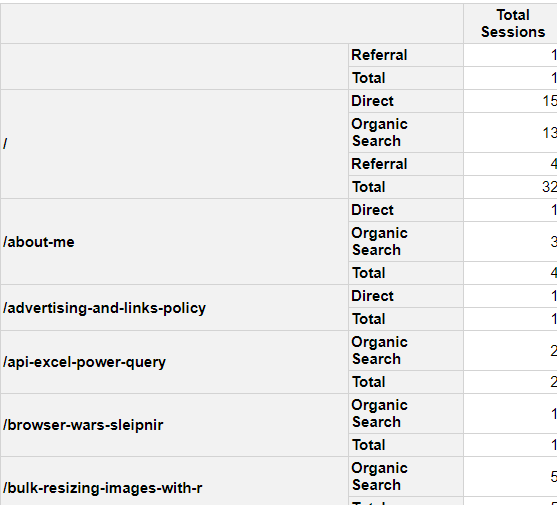
As you can see, it gives us a simple html output, which looks quite pretty and can be exported as an image or HTML like so.

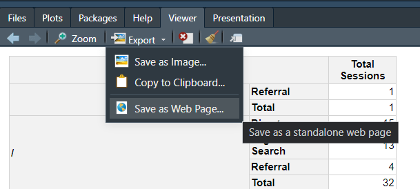
How to export an R pivot table to HTML from RStudio

Now, let’s have a look at how our R pivot table works.

How The R Pivot Table Works

Here’s that phrase again: let’s break it down:

pt1 <- PivotTable$new(): We’re creating an object called pt1, using a PivotTable function and creating a “new” column
pt1$addData(gaData): We’re invoking our dataset with our pivot table. The gaData frame in this case
pt1$defineCalculation(calculationName = “Total Sessions”, summariseExpression = “sum(Sessions)”): This tells R that the calculation we want to use for our pivot table is called “Total Sessions” and we’re using the sum calculation on “Sessions” from our dataset
pt1$addRowDataGroups(“Landing.page”): The first row of our pivot table, the “key”, is our landing page
pt1$addRowDataGroups(“Session.default.channel.group”): Our second column, our drilldown dimension, is our traffic channel
pt1$renderPivot(): Now we’re using pivottabler’s renderPivot command to turn this to HTML and render it in our viewer window

Adding Extra Columns To Our R Pivot Table

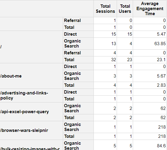
If you export directly from GA4, or you add extra metrics to your Google Analytics call (I promise I’ll update part 2 to use the GA4 API soon), you’ll find that you have metrics other than sessions, such as Users and Engagement Time.

Let’s add those to our pivot table as well, summing Users and calculating the Average Engagement Time, so we can see how many users our sessions are driving and how long they’re spending with our content from each channel.

We can do that like so:

pt2 <- PivotTable$new()
pt2$addData(gaData)
pt2$defineCalculation(calculationName = "Total Sessions", summariseExpression = "sum(Sessions)")
pt2$defineCalculation(calculationName = "Total Users", summariseExpression = "sum(Users)")
pt2$defineCalculation(calculationName = "Average Engagement Time", summariseExpression = "round(mean(Average.engagement.time.per.session), 2)")
pt2$addRowDataGroups("Landing.page")
pt2$addRowDataGroups("Session.default.channel.group")
pt2$renderPivot()

And that will give us the following output:

How This Expanded Pivot Table Works

I won’t re-use all the explanations from the previous section, but let’s take a look at the extra rows we’ve added. For clarity’s sake in the code, I’ve called this one “pt2” rather than “pt1”.

pt2$defineCalculation(calculationName = “Total Users”, summariseExpression = “sum(Users)”): We’ve added an extra column to our pivot table called “Total Users”, which is adding up “Users” from our gaData dataset
pt2$defineCalculation(calculationName = “Average Engagement Time”, summariseExpression = “round(mean(Average.engagement.time.per.session), 2)”): This line might look a little intimidating, but all it’s doing is calculating the Average Engagement Time, and then using the round function to take it to two decimal places, which is why it’s wrapped in brackets

So there we go. Hopefully that gives you a solid basis to create pivot tables in R.

Let’s look at styling them up so that you can include them in presentations and share with your clients.

Adding Styling To Pivot Tables With R

Finally, let’s create another pivot table using our R code from earlier, but naming it p3 instead of p2. From here, we’ll add another few lines to style our cell backgrounds in dark green (the accent colour from my site).

Here’s how to do that:

pt3 <- PivotTable$new()
pt3$addData(gaData)
pt3$defineCalculation(calculationName = "Total Sessions", summariseExpression = "sum(Sessions)")
pt3$defineCalculation(calculationName = "Total Users", summariseExpression = "sum(Users)")
pt3$defineCalculation(calculationName = "Average Engagement Time", summariseExpression = "round(mean(Average.engagement.time.per.session), 2)")
pt3$addRowDataGroups("Landing.page")
pt3$addRowDataGroups("Session.default.channel.group")
pt3$evaluatePivot()

### Add Styling

pt3$setStyling(
  rowNumbers = c(1),  # Target the header row
  columnNumbers = c(4, 5, 6),  # Target the specific columns
  declarations = list("text-align" = "centre", "color" = "#008285")
) 
pt3$renderPivot()

Let’s take a look at the extra rows and how the styling works.

How Styling In Pivottabler Works

For the last time today, let’s break it down:

pt3$setStyling(: We’re telling R to apply styling rules
rowNumbers = c(1): We’re looking at the first row, the header row containing the column names
columnNumbers = c(4, 5, 6): These are the columns for “Total Users”, “Average Engagement Time”, and “Total Sessions”
declarations = list(“text-align” = “center”): Here, we’re setting the above columns to be centre aligned
“color” = “#F46239”)): Finally, we’re setting the accent colour to the same colour as my site’s accent colour – change as appropriate

And there we go, a whistlestop tour of using the SEO’s old favourite – pivot tables – in R with Google Analytics data and adding some styling to it. Try it yourself, there’s a lot you can do with them.

Wrapping Up

That’s a few common Excel formulas replicated with R, how to create pivot tables and to style them up according to your branding.

I hope you’ll join me next time, where we’ll take a look at using APIs in R. I’m really excited about that piece, and I hope you’ll enjoy reading it and using it as much as I enjoyed writing it.

As always, our R script is below.

Our Code From Today

# Install Packages

library(tidyverse)

library(rvest)

library(pivottabler)

# Read Search Console Queries

gscData <- read.csv("Queries.csv", stringsAsFactors = FALSE)

# If Statement for >= 50 Impressions

gscData$Fifty.Or.More.Impressions <- ifelse(gscData$Impressions >=50, "YES", 
                                            "NO")

# If Else Statement With Multiple Conditions

gscIFELSE1 <- if(gscData$Impressions[1] >=50){
  return("Greater or Equal")
}else{
  return("Less")
}

## If Else Statement Function

gscIFELSEFun <- function(x, y){
  
  if(x >= y){
    return("Greater or Equal")
  }else{
    return("Less")
  }
  
}

gscData$Function <- sapply(gscData$Impressions, gscIFELSEFun, 50)

## Nested If Else Statement Function

gscNestedFun <- function(x, y){
  
  if(x > y){
    return("Greater")
  }else{
    if(x < y){
      return("Less")
    }else{
      if(x == y){
        return("Equal")
      }
    }
  }
}

gscData$NestedFunction <- sapply(gscData$Impressions, gscNestedFun, 50)

# Excel Countif In R

sum(gscData$Impressions >= 50, na.rm=TRUE)

# Excel Sumif In R

sum(gscData$Impressions[gscData$Impressions >= 50])

# Excel Index Match In R

## TV Unit Data & Domain Function From Part 4

tvUnits <- read.csv("tvUnits.csv", stringsAsFactors = FALSE)

domainNames <- function(x){
  
  strsplit(gsub("http://|https://|www\\.", "", x), "/")[[c(1, 1)]]
  
}

tvUnits2 <- data.frame(tvUnits$URL)

names(tvUnits2) <- names(tvUnits["URL"])

tvUnits2$Domain <- sapply(tvUnits2$URL, domainNames)

## Index Match Emulation With Left_Join

tvUnits$Domain <- tvUnits %>% 
  left_join(tvUnits2, by = "URL")

## Index Match Emulation Function Without Dplyr

indexMatch <- function(x, y, z){
  
  row <- match(x, y)
  
  targetVal <- z[row]
  
}

tvUnits$Domain2 <- indexMatch(tvUnits$URL, tvUnits2$URL, tvUnits2$Domain)

# Pivot Tables In R

gaData <- read.csv("gaData.csv", stringsAsFactors = FALSE)

## First Pivot Table

pt1 <- PivotTable$new()
pt1$addData(gaData)
pt1$defineCalculation(calculationName = "Total Sessions", summariseExpression = "sum(Sessions)")
pt1$addRowDataGroups("Landing.page")
pt1$addRowDataGroups("Session.default.channel.group")
pt1$renderPivot()

## Second Pivot Table With Extra Metrics 

pt2 <- PivotTable$new()
pt2$addData(gaData)
pt2$defineCalculation(calculationName = "Total Sessions", summariseExpression = "sum(Sessions)")
pt2$defineCalculation(calculationName = "Total Users", summariseExpression = "sum(Users)")
pt2$defineCalculation(calculationName = "Average Engagement Time", summariseExpression = "round(mean(Average.engagement.time.per.session), 2)")
pt2$addRowDataGroups("Landing.page")
pt2$addRowDataGroups("Session.default.channel.group")#pt2$renderPivot()

## Styling Pivot Table

pt3 <- PivotTable$new()
pt3$addData(gaData)
pt3$defineCalculation(calculationName = "Total Sessions", summariseExpression = "sum(Sessions)")
pt3$defineCalculation(calculationName = "Total Users", summariseExpression = "sum(Users)")
pt3$defineCalculation(calculationName = "Average Engagement Time", summariseExpression = "round(mean(Average.engagement.time.per.session), 2)")
pt3$addRowDataGroups("Landing.page")
pt3$addRowDataGroups("Session.default.channel.group")
pt3$evaluatePivot()
###Add Styling
pt3$setStyling(
  rowNumbers = c(1),  # Target the header row
  columnNumbers = c(4, 5, 6),  # Target the specific columns
  declarations = list("text-align" = "centre", "color" = "#008285")
) 
pt3$renderPivot()

R For SEO Part 5: Common Excel Formulas In R

The Ifelse Statement In R

The Anatomy Of An Ifelse Command In R

If Else In R With Multiple Conditions

How Our If Else R Function Works

Nesting If Else Statements To Replicate Excel IFS Formula In R

Excel Countif In R

Excel Sumif In R

How Sumif Replication In R Works

Index Match Or Vlookup In R

Preparing Our Dataset For Index Match/ Vlookup Emulation With R

Index Match Or Vlookup In R With Left_Join

An Index Match Function In R Without Dplyr

How The IndexMatch Function Works

Pivot Tables In R

Our First Pivot Table With Pivottabler

How The R Pivot Table Works

Adding Extra Columns To Our R Pivot Table

How This Expanded Pivot Table Works

Adding Styling To Pivot Tables With R

How Styling In Pivottabler Works

Wrapping Up

Our Code From Today

Ben Johnston

Pages

Newsletter

The Ifelse Statement In R

The Anatomy Of An Ifelse Command In R

If Else In R With Multiple Conditions

How Our If Else R Function Works

Nesting If Else Statements To Replicate Excel IFS Formula In R

Excel Countif In R

Excel Sumif In R

How Sumif Replication In R Works

Index Match Or Vlookup In R

Preparing Our Dataset For Index Match/ Vlookup Emulation With R

Index Match Or Vlookup In R With Left_Join

An Index Match Function In R Without Dplyr

How The IndexMatch Function Works

Pivot Tables In R

Our First Pivot Table With Pivottabler

How The R Pivot Table Works

Adding Extra Columns To Our R Pivot Table

How This Expanded Pivot Table Works

Adding Styling To Pivot Tables With R

How Styling In Pivottabler Works

Wrapping Up

Our Code From Today

Related Posts

Ben Johnston

Pages

Newsletter

Follow Me